CUDA Path Tracer with À-Trous Denoiser

- Tested on: Ubuntu 20.04 LTS, Ryzen 3700X @ 2.22GHz 48GB, RTX 2060 Super @ 7976MB
CUDA Path Tracer
Highlights
Finished path tracing core features:
- diffuse shaders
- perfect specular reflection
- 1st-bounce ray intersection caching
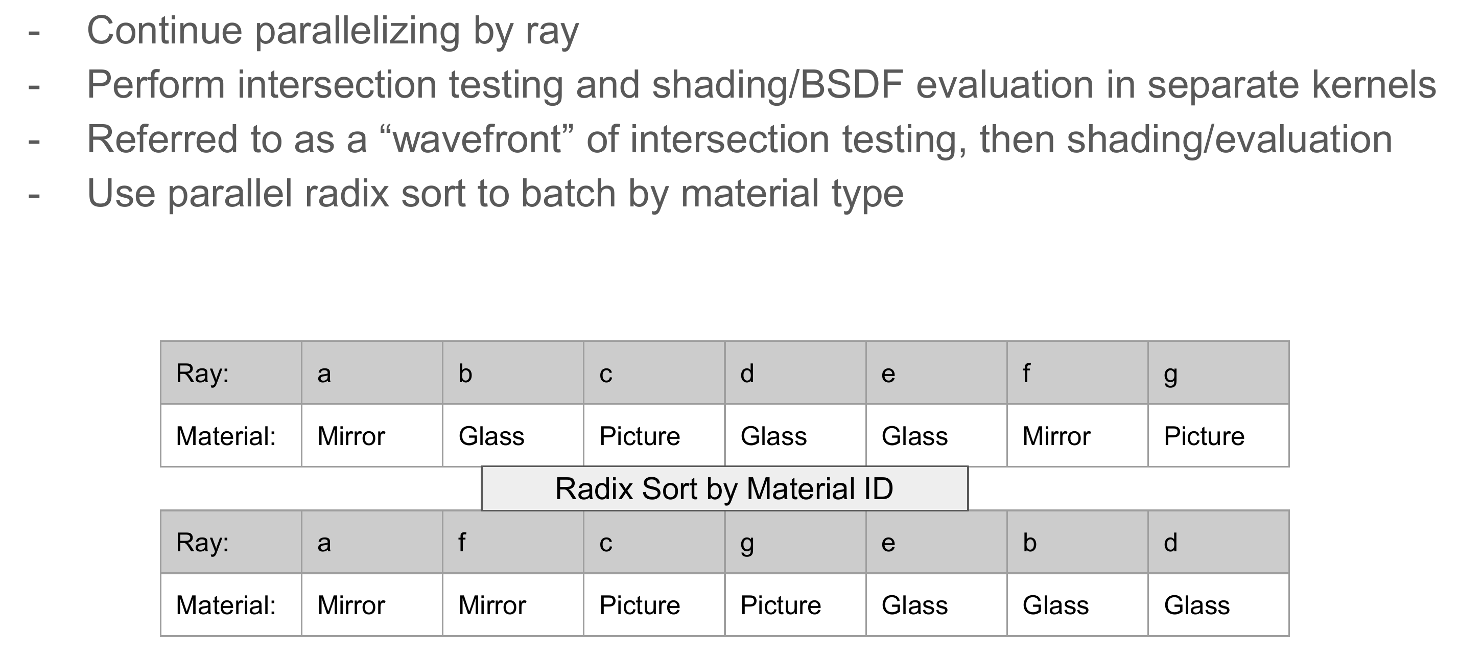
- radix sort by material type
- path continuation/termination by Thrust stream compaction
Finished Advanced Features:
- Refraction with Fresnel effects using Schlick’s approximation
- Stochastic sampled anti-aliasing
- Physically-based depth of field
- OBJ mesh loading with tinyobjloader
Background: Ray Tracing
Ray tracing is a technique commonly used in rendering. Essentially it mimics the actual physical behavior of light: shoots a ray from every pixel in an image and calculates the final color of the ray by bouncing it off on every surface it hits in the world, until it reaches the light source. In practice a maximum number of depth (bouncing times) would be specified, so that we would not have to deal with infinitely bouncing rays.
Ray tracing is one of the applications considered as “embarrassingly parallel”, given the fact that each ray is completely independent of other rays. Hence, it is best to run on an GPU which is capable of providing hundreds of thousands of threads for parallel algorithms. This project aims at developing a CUDA-based application for customized ray tracing.
BSDF: Bidirectional Scattering Distribution Functions
BSDF is a collection of models that approximates the light behavior in real world. It is commonly known to consist of BRDF (Reflection) models and BTDF (Transmission) models. Some typical reflection models include:
- Ideal specular (perfect mirror,
glm::reflect) - Ideal diffuse. It is a model that the direction of the reflected ray is randomly sampled from the incident hemisphere, along with other advanced sampling methods.
- Microfacet, such as Disney model.
- Glossy specular.
- Subsurface scattering.
- …
Some typical transmission models include:
- Fresnel effect refraction. It consists of a regular transmission model based on Snell’s law and a partially reflective model based on Fresnel effect and its Schlick’s approximations.
- …
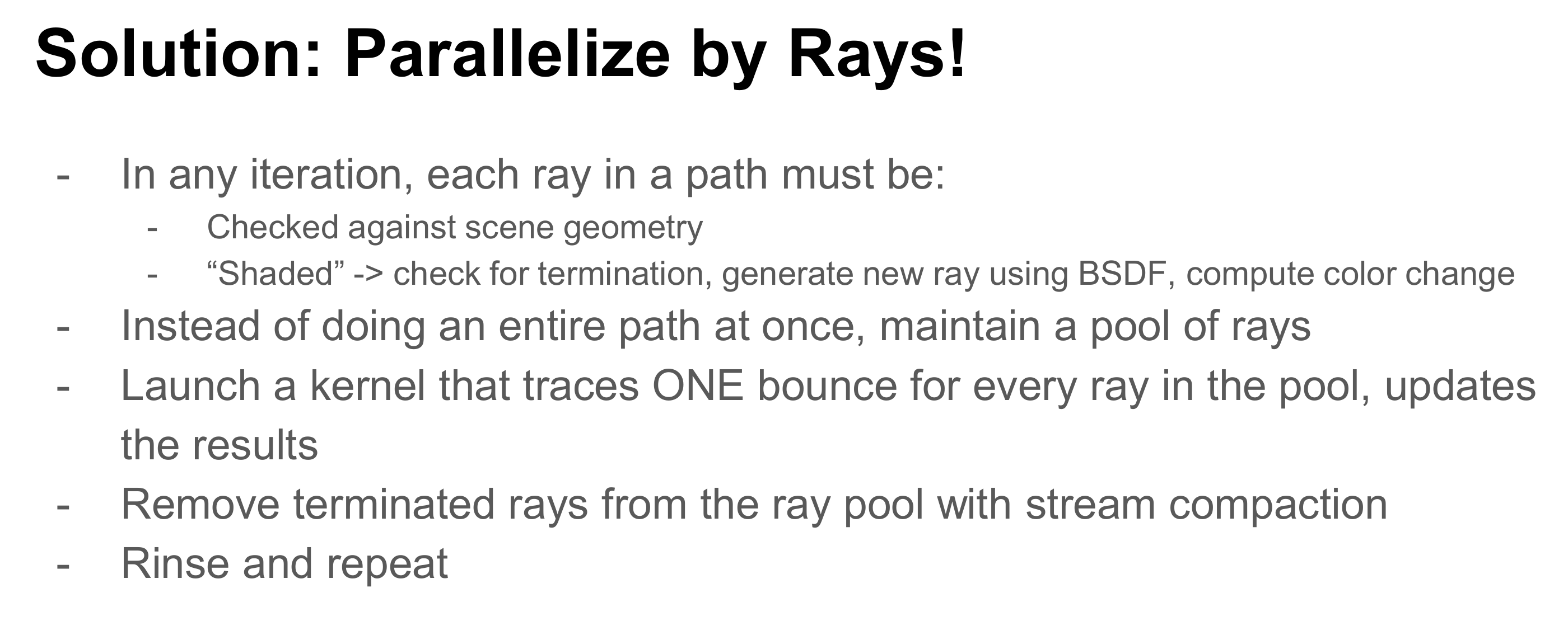
CUDA Optimization for Ray Tracing
In order to better utilize CUDA hardware for ray tracing, it is not suggested to parallelize each pixel, as it would lead to a huge amount of divergence.
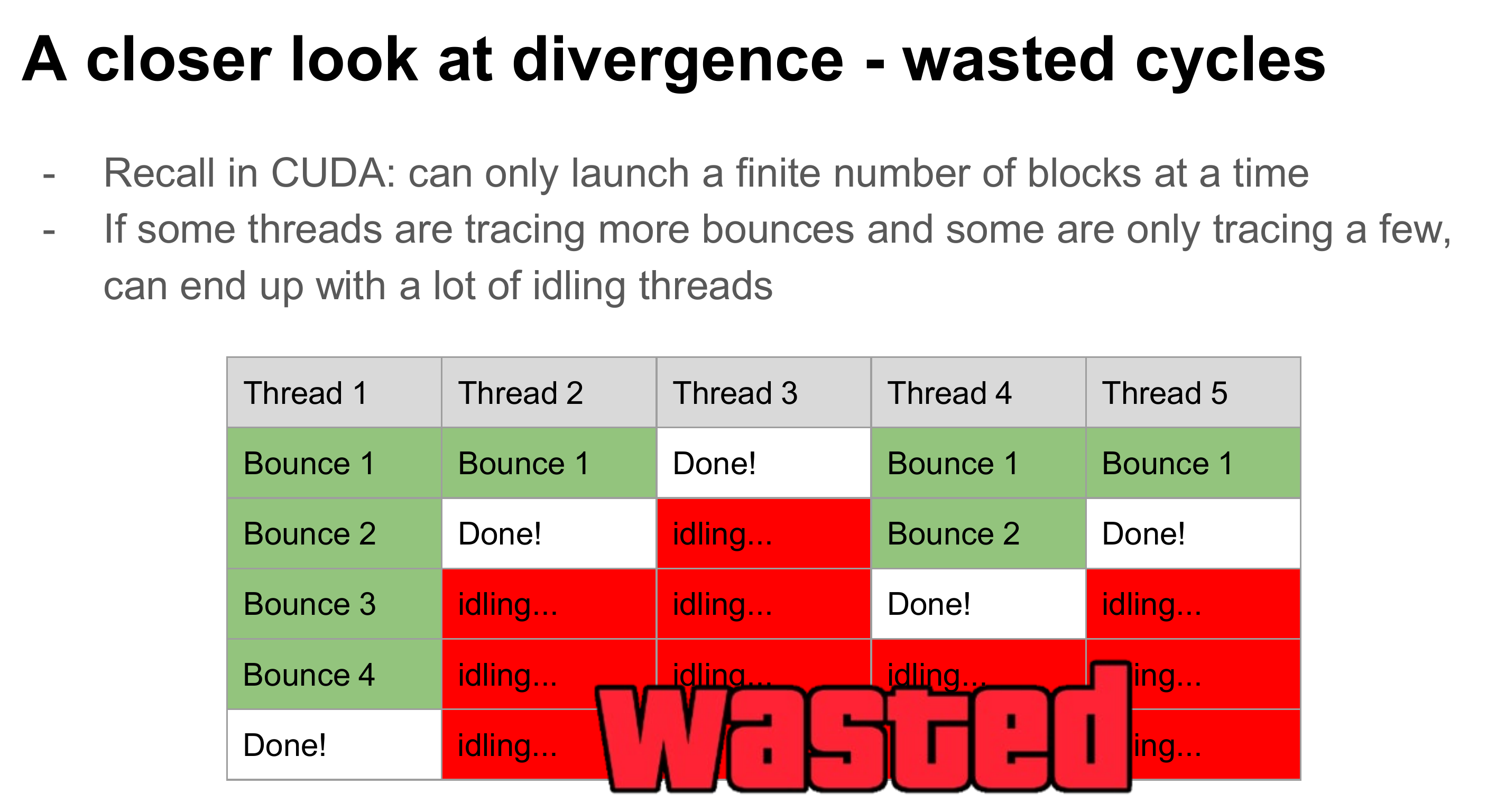
Instead, one typical optimization people use is to parallelize each ray, and uses stream compaction to remove those rays that terminates early. By this means we could better recycle the early ending warps for ray tracing other pixels.
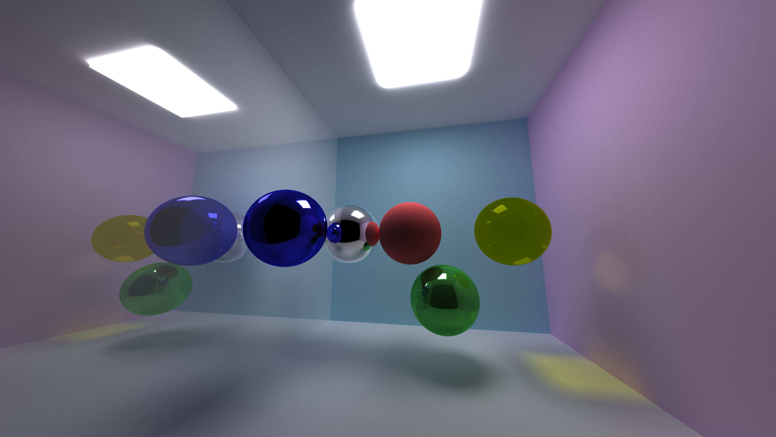
Results and Demos
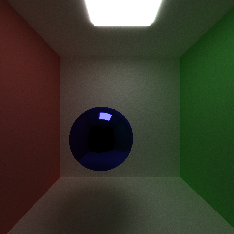
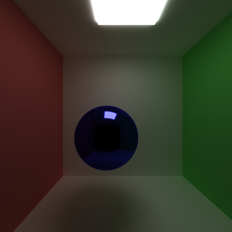
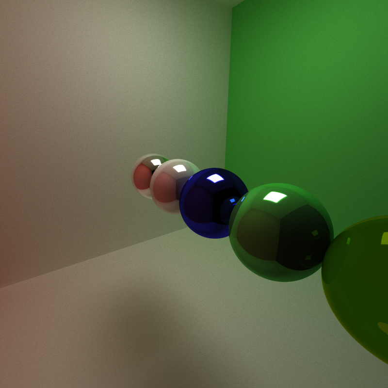
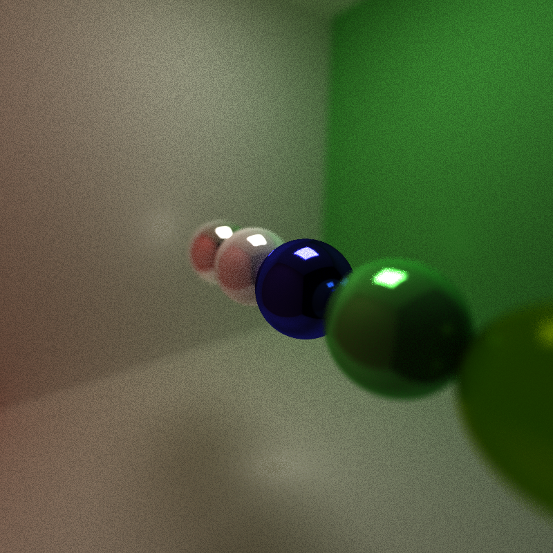
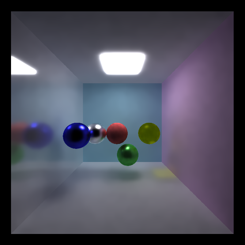
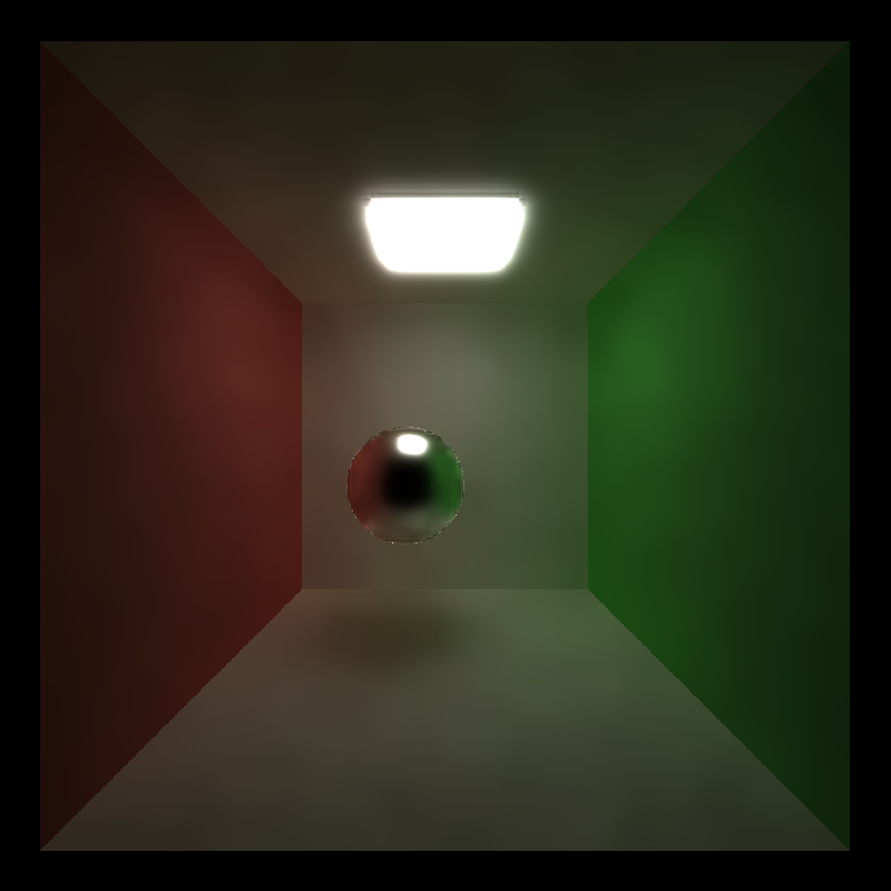
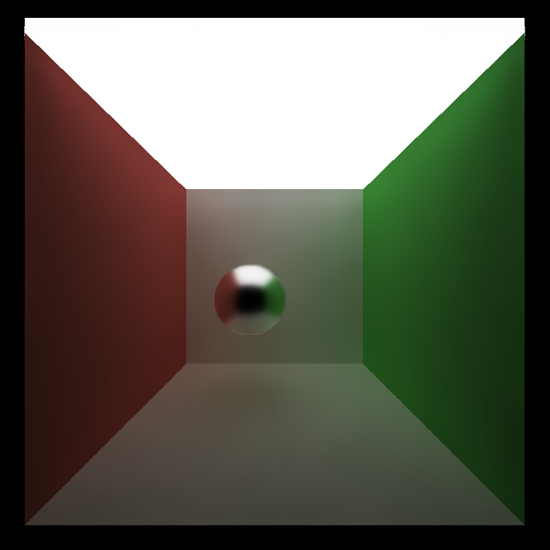
Ray Refraction for Glass-like Materials
| Perfect Specular Reflection | Glass-like Refraction |
|---|---|
 | 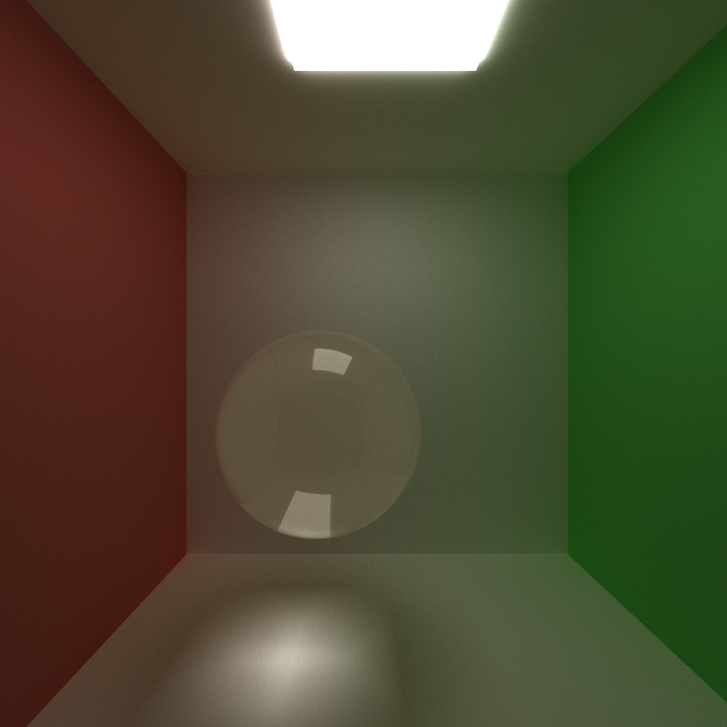 |
Stochastic Sampled Anti-Aliasing
| 1x Anti-Aliasing (Feature OFF) | 4x Anti-Aliasing |
|---|---|
 |  |
Physically-Based Depth of Field
| Pinhole Camera Model (Feature OFF) | Thin-Lens Camera Model |
|---|---|
 |  |
Mesh Loading
Mesh loading has not been fully supported due to an incorrect normal vector parsing issue in tinyobjloader. The runtime is also unoptimized and takes an unreasonable amount of time to run.
TODO:
- Bounding volume culling with AABB box/OBB box.
Performance Analysis
Throughout the project two optimizations were done:
- Cache ray first bounce. For every iteration in a rendering process, the first rays that shoot from camera to the first hit surface is always the same. Therefore we can cache the first shooting ray during the first iteration and reuse the results in all the following iterations.
- Radix-sort hit attributes by material type. The calculation of resulting colors for each ray depends on the material of the object it hits, and thus we can sort the rays based on material type before shading to enforce CUDA memory coalescence.
The following experiments are conducted on a Cornell box scene as shown in cornell_profiling.txt with varying iterations from 300 to 2000.
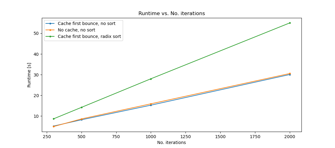
From the performance analysis we can see that caching the first bounce for the 1st iteration has a slight improvement on the performance, while radix-sorting the material type before shading have a great negative impact on the performance. This is possibly due to the reason that radix-sorting itself takes a lot amount of time in each iteration.
CUDA Denoiser
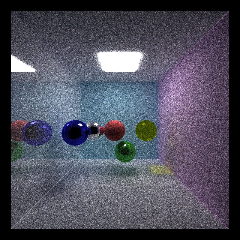
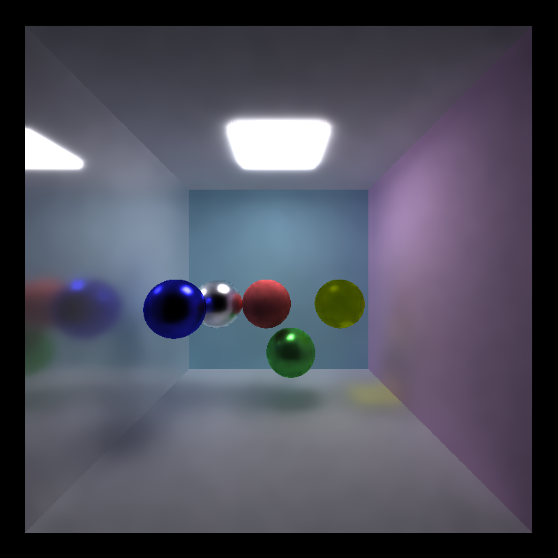
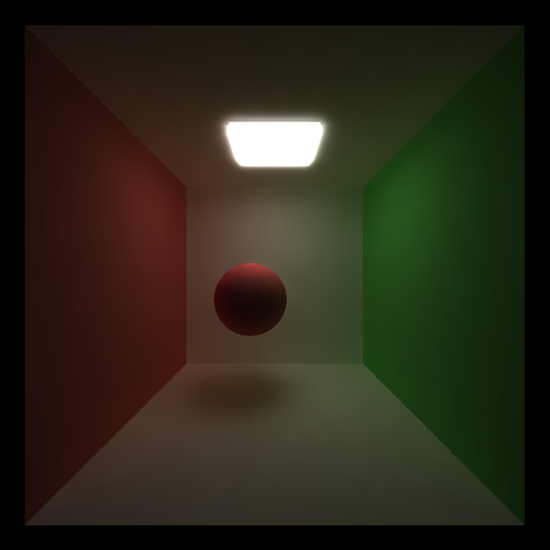
Physically-Based Ray Traced (PBRT) Image with À-Trous Denoising
| PBRT, 5000 iterations | PBRT, 5000 iterations, 4x anti-aliasing |
|---|---|
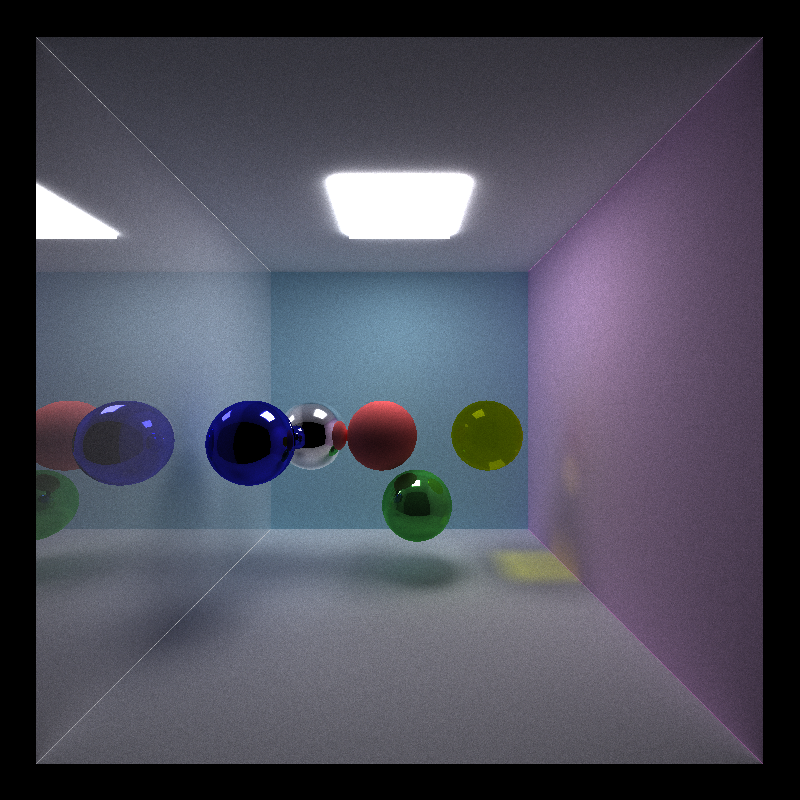 |  |
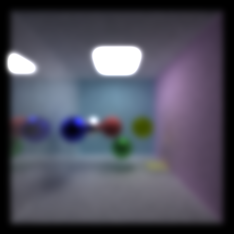
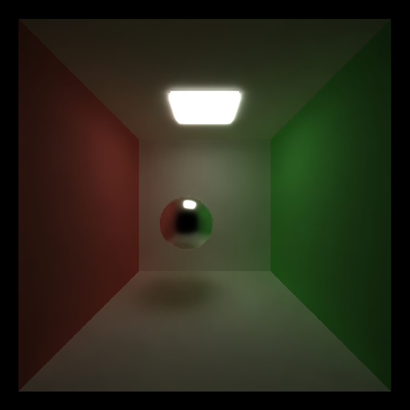
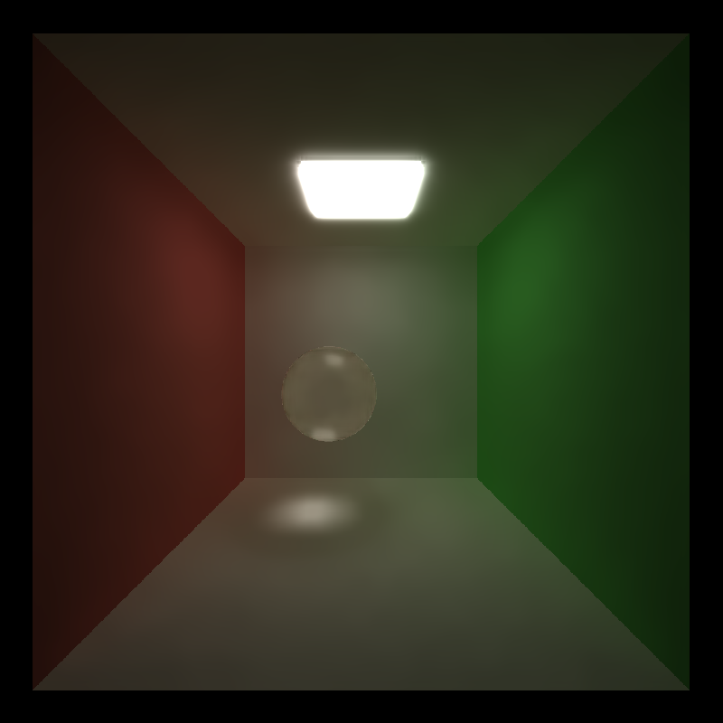
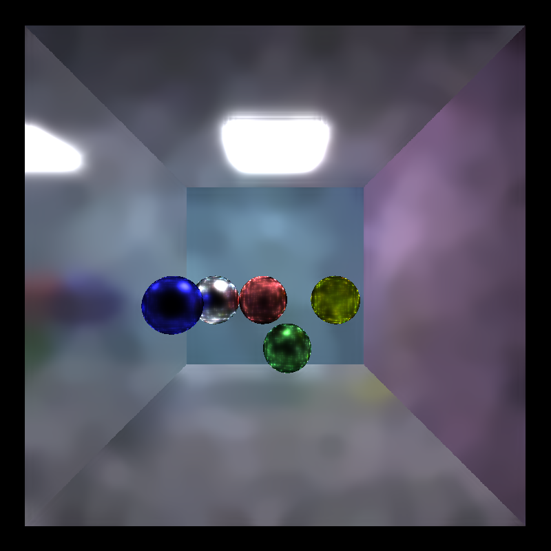
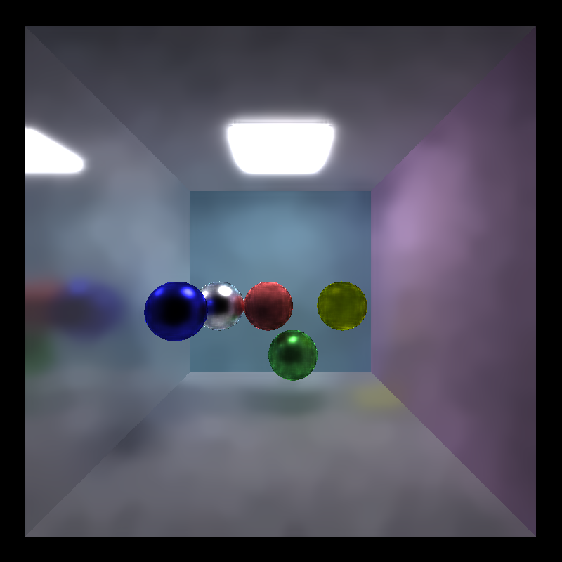
| PBRT, 100 iterations | PBRT, 100 iterations, À-Trous Denoising |
|---|---|
 |  |
Highlights
Implemented Edge-Avoiding À-Trous Wavelet Transform denoising techniques with 5x5 Gaussian blur kernel.
Introduction
Physically-Based Ray Tracing (PBRT) is considered as one of the best methods that produce the most photorealistic images. The essence of PBRT is to approximate the rendering equation with Monte-Carlo integration, sampling multiple rays from each pixel of an image and bouncing them off multiple times from various surfaces of different kinds and different textures according to the ray directions, accumulating the colors along the way.
However, in reality it is very hard to run PBRT in real time, as we often need a large amount of rays to obtain a reasonable good approximation for the rendering equation. Hence, people come up with multiple ways of applying denoising techniques on partially ray-traced images, hoping that with denoising we could get reasonably good photorealistic images while terminating PBRT early. In this project, we explored Edge-Avoiding À-Trous Wavelet Transform for image denoising. For more details, please checkout the project instruction.
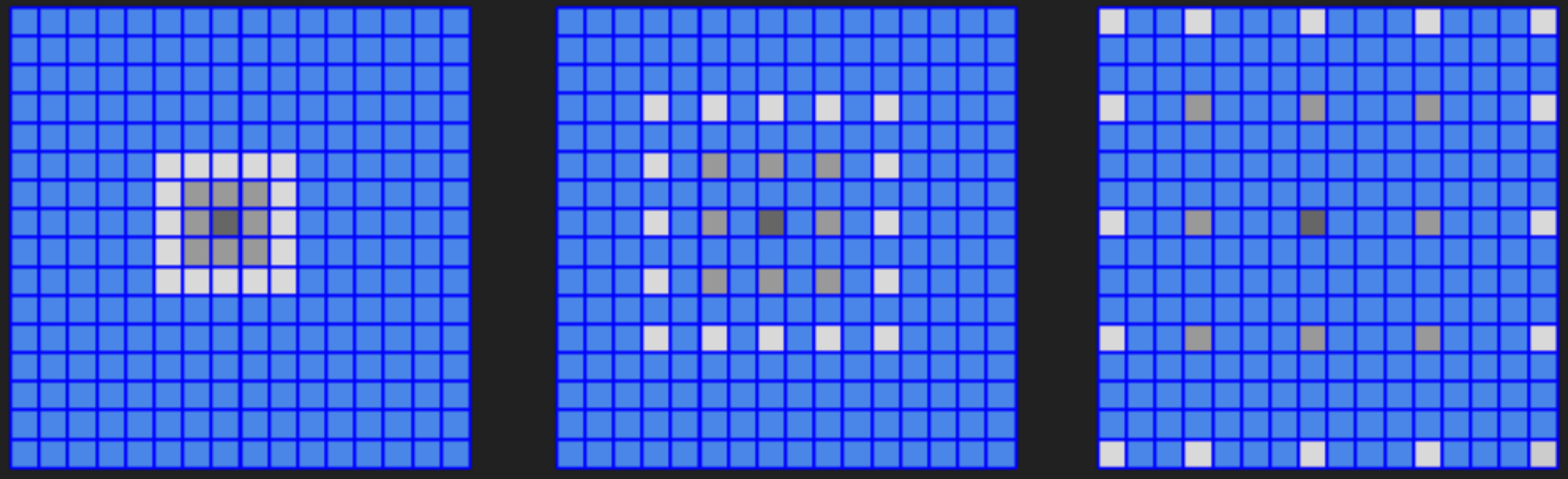
The word “À-Trous” with meaning “with holes” comes from Algorithme À-Trous, which is a stationary wavelet transform commonly used in computer graphics to approximate the effect of a Gaussian filter with much faster performance. It starts from a fix-sized Gaussian filter, performs convolution on the image while expanding out each element of the filter at every iteration, filling all missing entries with 0s. The “Edge-Avoiding” part of the algorithm incorporates the use of a pixel-wise GBuffer, storing positions and normals of the first hit for each ray. When the image is denoised, information of the GBuffer will be used to avoid blurring edges in the image, while the noisy surfaces are smoothed.
| Pure À-Trous Filtering | À-Trous Filtering with Edge-Avoiding GBuffer |
|---|---|
 |  |
Qualitative Analysis
Visual Results vs. Filter Size
The following experiments are run with c_phi=132.353, n_phi=0.245, p_phi=1.324.
| Filter Size = 6 | Filter Size = 15 | Filter Size = 32 | Filter Size = 100 |
|---|---|---|---|
 |  |  |  |
From the results we can see that the visual results does not vary uniformly with the filter size. When the filter reaches some size threshold, it is no longer the filter size that stops the smoothing process but the weights of the GBuffer instead.
Visual Results vs. Material Type
The following experiments are run with c_phi=132.353, n_phi=0.245, p_phi=1.324, filter_size=100.
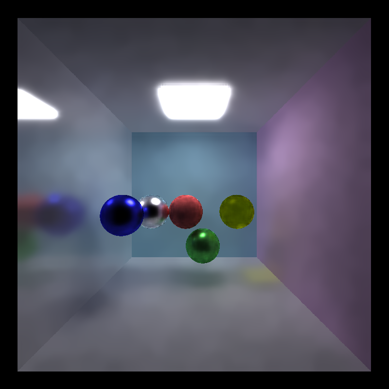
| Diffuse | Reflective | Refractive |
|---|---|---|
 |  |  |
From the results we can see that the filter works best with diffuse materials, reasonably well with refractive materials, and the worst with reflective materials. This is mainly because the current implementation only caches the position & normal vectors of the first hit, while this property does not really apply to reflective materials (colors on a pure-reflective material depend heavily on the material properties from the 2nd hit). As a result, the filter is blurring the reflection on the reflective materials.
Visual Results vs. Light Conditions
The following experiments are run with c_phi=132.353, n_phi=0.245, p_phi=1.324, filter_size=100.
| Cornell Box | Cornell Box with Large Lights |
|---|---|
 |  |
From the results we can see that the filter works better in brighter lighting conditions. This is because in brighter lighting conditions the color tends to be more similar locally, while with point lights the color differs much from its adjacent pixels, making it more difficult to smooth.
Quantitative Analysis
Denoising Time
For a standard scene as shown in Physically-Based Ray Traced (PBRT) Image with À-Trous Denoising, the denoising time for a 800x800 image with c_phi=132.353, n_phi=0.245, p_phi=1.324, filter_size=100 is:
----- Begin image denoising -----
   elapsed time: 31.2983ms    (CUDA Measured)
which is a reasonably fast denoising time.
Number of Iterations Needed for a Smooth Image
The following experiments are run with c_phi=132.353, n_phi=0.245, p_phi=1.324, filter_size=100.
| Iteration = 1 | Iteration = 10 | Iteration = 25 |
|---|---|---|
 |  |  |
| Iteration = 50 | Iteration = 100 |
|---|---|
 |  |
From the results we can see that subjectively, with the parameters specified above, we can get a reasonably smooth image with number of iterations at least 50.
Denoising Runtime vs. Resolution, Filter Size
The following experiments are run with c_phi=132.353, n_phi=0.245, p_phi=1.324. For varying resolution, filter_size = 100; for varying filter size, resolution = 800x800.
| Runtime vs. Resolution | Runtime vs. Filter Size |
|---|---|
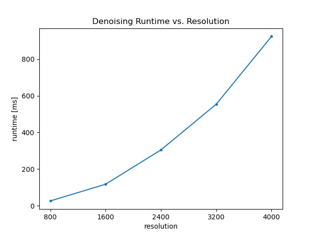 | 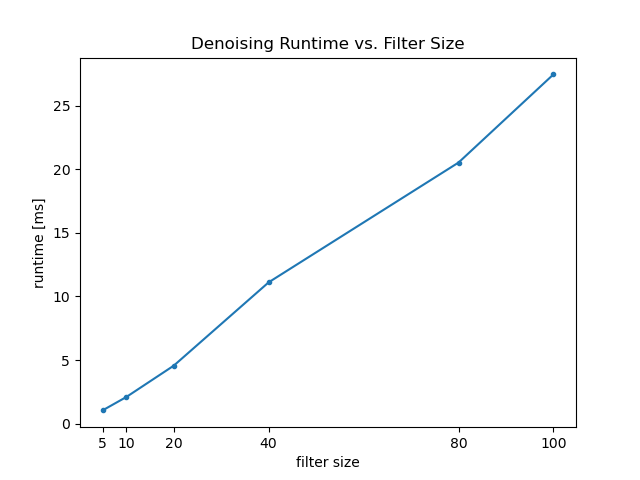 |
From the results we can see that the runtime increases quadratically with resolution as the number of pixels increases quadratically with resolution; the runtime increases linearly with filter size, as increasing filter size would only increase the number of iterations that À-Trous wavelet transform needs to run.
References
- [PBRT] Physically Based Rendering, Second Edition: From Theory To Implementation. Pharr, Matt and Humphreys, Greg. 2010.
- Antialiasing and Raytracing. Chris Cooksey and Paul Bourke, http://paulbourke.net/miscellaneous/aliasing/
- Sampling notes from Steve Rotenberg and Matteo Mannino, University of California, San Diego, CSE168: Rendering Algorithms
- Path Tracer Readme Samples (non-exhaustive list):
- https://github.com/byumjin/Project3-CUDA-Path-Tracer
- https://github.com/lukedan/Project3-CUDA-Path-Tracer
- https://github.com/botforge/CUDA-Path-Tracer
- https://github.com/taylornelms15/Project3-CUDA-Path-Tracer
- https://github.com/emily-vo/cuda-pathtrace
- https://github.com/ascn/toki
- https://github.com/gracelgilbert/Project3-CUDA-Path-Tracer
- https://github.com/vasumahesh1/Project3-CUDA-Path-Tracer
- Edge-Avoiding A-Trous Wavelet Transform for fast Global Illumination Filtering
- Spatiotemporal Variance-Guided Filtering
- A Survey of Efficient Representations for Independent Unit Vectors
- ocornut/imgui - https://github.com/ocornut/imgui