My F1TENTH Journey — Lab 4, Reactive Planning Methods for Obstacle Avoidance

This series of blogs marks the journey of my F1/10 Autonomous Racing Cars.
All my source codes can be accessed here.
Previous post:
- My F1TENTH Journey — Lab 1, Introduction to ROS
- My F1TENTH Journey — Lab 2, Automatic Emergency Braking
- My F1TENTH Journey — Lab 3, PID-Controlled Wall Follower
Overview
Obstacle avoidance is one of the critical parts of autonomous driving. Crashing into obstacles could possibly bring serious damages to both the car and the object that it runs into. Overtime, researchers and developers have come up with multiple ways to avoid obstacles. This lab focuses on implementing a reactive way (also passive way) of avoiding obstacles to drive the car around in free space, provided with only real-time 2D LiDAR sensor data.
“Follow the Gap” Algorithm
With 2D laser scan data, we can easily tell whether there is an obstacle in front of us by looking into the range (length) of each beam. If the range of a certain beam is small, we know that the laser travelling in this direction hits an obstacle in close range; conversely, if the range of a beam is large, we know that the laser beam is able to travel very far before hitting on an obstacle, and thus we can consider this direction as “free space”. “Follow the Gap” algorithm states that, for each incoming LaserScan LiDAR data, we first figure out the direction of the closest obstacle, and then try to maneuver the vehicle in the direction of “free space” to avoid this obstacle.
In theory, “Follow the Gap” planner can be done in the several steps:
- Find the nearest LiDAR endpoint and put a “safety bubble” of radius $r$ around it.
- Set all endpoints inside the bubble to distance $0$. All non-zero endpoints are considered “free space”.
- Find maximum length sequence of consecutive non-zero endpoints and identify the “widest” free space. (The max-gap.)
- Choose the furthest endpoint in the max-gap, and steer the vehicle in that direction with some certain speed.
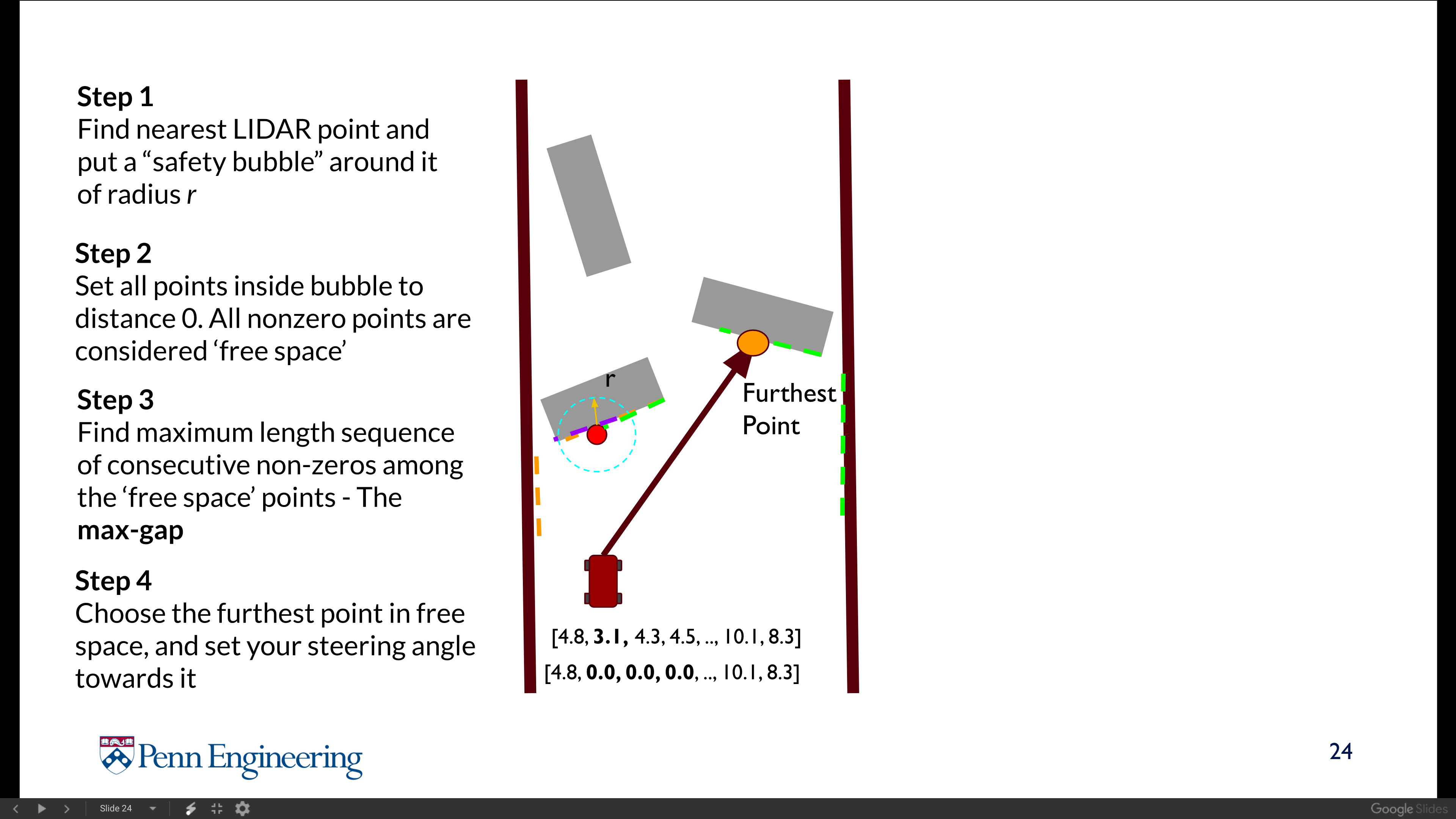
‘Follow the Gap’ Algorithms in diagrams.
Notes in Real Practice
- Laser scan data must be smoothed and de-noised.
In actual implementation, we can never obtain a clean laser scan data from LiDAR sensor. Due to hardware issues the raw data would contain lots of noises and glitches. To smooth the data, I applied a sliding window of size 5 to average out each of the endpoints. I also clip the data within [range_min, range_max) according to the parameters in the incoming LaserScan ROS message.
- Calculate the distance between two laser scan endpoints with trigonometric formulas.
In the algorithm we wish to draw a “safety bubble” around the nearest endpoint by traversing all laser beams and setting all endpoints within the radius of that bubble to $0$. But with laser scan data, how can we compute the distance between two endpoints? Trigonometry provides us with a power tool called the Law of Cosines. With laser beams of range $r_1,r_2$ and their angle $\theta$, we can draw a triangle among the vehicle, endpoint 1, endpoint 2, and apply: $$d=\sqrt{r_1^2+r_2^2-2r_1r_2\cos\theta},$$ which gives us the distance between the two endpoints.
- Impose a “safety angle” around the safety bubbles.
One of the corner case in testing the algorithm is the corner of the wall. As the figure indicates below, the car detects the corner of the wall and has marked it as an obstacle, setting all points within the safety bubble as 0. However, the laser beam direction that detects the farthest endpoint in the max-gap happens to be right next to the obstacle, causing the car to make a left turn rather than right turn, and directly hits the wall.
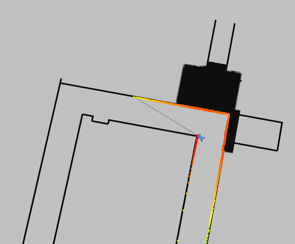
Demonstration of a corner case without safety angle.
To address this issue, I added a “safety angle” around the bubble, which basically sets the laser beams too close to the direction of obstacles to distance 0. For instance, a safety angle of 20 degrees would set additional laser beams in the direction leftwards of the bubble by 20 degrees and rightwards of that bubble by 20 degrees also to 0. This simple method would prevent the vehicle to get too close to the obstacle, even if the best direction of free space happens to be next to the obstacle.
Demo Videos
References
F1/10 Autonomous Racing Lecture: Reactive Methods for Planning